Happy Pi Day!
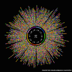
Here’s a picture visualizing the digits in Pi.
Remember, there is nothing universal about a base-10 numbering system. So, while this graph sure has some perdy colors in it, it’s mostly meaningless. But, that’s the beauty of irrational numbers: il y a un peu de je ne sais quoi.
But hey! look a STAR!
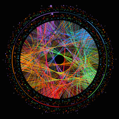
This one visualizes the relationships between digits in pi.
Again, it’s a meaningless representation of the data since it’s visualizing the base-10 numbering system. The star shows up in the picture because there are 10 digits and the artist chose to alternate between light and dark! If we did the same thing with a base 14 numbering system, you’d see a 7 pointed star… Look at the colors though! The colors!
Back to the Bioinformatics Algorithms
These are the algorithms I’m most proud of implementing. Sure, this code is available on github, but it’s written in Clojure, so it’s impossible for most people to understand without some head-scratching. In fact, it took quite a bit of effort just for me to freshen up enough to write this article. And that, my friends, is security by obfuscation – which is not a virtue for code or for much of anything, really.
I enjoy writing code in Clojure because Lisp forces you to write code in a functional manner and therefore your code more closely resembles the pure math you’re implementing. I’ve been sending out this project along with job applications, but I don’t think most people understand what they’re looking at, which is unfortunate. So, I’ve blogged about it and I’ll send out this link instead.
I can’t imagine that someone else hasn’t thought of these ideas for bioinformatics. Sure, they involve some bitcrunching, but it’s really not that complicated. Specifically, here are the two algorithms in my project that I’m referring to.
★ Constant Time Hamming Distance implemented specifically for strings of nucleotides.
★ Neighbor Transform. Basically, simultaneous binary addition, specifically for nucleotides.
Bioinformatics on Coursera
Back in November, I started taking this Bioinformatics class on Coursera, taught by Pavel Pevzner and Phillip Compeau. It was one of the best classes I’ve taken on Coursera so far. The interactive text was very well built and organized. I could progress without needing to watch the videos, but those were a great resource if I needed more detail in some sections.
Additionally, the course was just the right level of challenging: not only did you have to write the code, but your submissions were automatically graded with a five minute time limit. And in bioinformatics, ** * time is key! * ** So if you couldn’t write your code to complete within that five minute time limit, you didn’t get any credit for those solutions. The problems were all great Computer Science algorithms: motif enumeration, hamming distance and a good bit of graph theory.
For their language of choice, most students went with Python, which is expected for university students. However, I solved the problems in Clojure :) and this made things both easier and harder. It was a bit harder to rethink these problems to properly utilize recursion, immutable data structures and other functional programming paradigms.
However, the consequences of doing so proved invaluable when my solutions were a bit too slow. Solution didn’t run within the time limit?! Oh shit, better completely rewrite my solution to include thread pools and …. wait, just kidding! r/fold and pmap that shit! LMAO. Needz moar threadz? No problem, I really just need more cores!
A side trek into supercomputing
And this, folks, is why the work that the great folks on HP’s team for The Machine will absolutely revolutionize computing in the next five years. It completely changes the software paradigm for supercomputing. Computing is going to start moving very fast: much faster than we anticipate! Because of revolutions in hardware that shift the paradigm of software, that means Moore’s Law – while still technically applicable until quantum/nano computing – no longer determines the limits of computing.

Because HP has patented all the things, their stock is going to be a good long term buy! =$
HP has patented several key technologies in it’s development of The Machine. Excluding the development of competing technologies (which isn’t very likely) or the complete collapse of the global economy, i’m extremely confident that HP is a good long term buy. As to how good, I can’t say. I would place another large bet on HP’s decision to restructure being fairly dependent on the development of this new technology =] =]
Watch this Video for a 7 Minute Overview of The Machine
Note: HP is restructuring itself into two public companies: one to sell PC’s to consumers and the other to sell servers and networking gear. Make sure you purchase the correct stock!
Fiber to the Dome
One of their game-changing technologies is photonics. Having phonotics integrated into the bus means that CPU’s are no longer physically bound to their memory. That’s an oversimplified explanation of things. However, as it is now, software developers for computationally intensive projects have to include lots of code just to push data where it’s needed. But photonics means that CPU’s can access a nearly unlimited supply of memory, instantaneously.
This means supercomputers and the software they run can begin to be designed very differently: you basically just need to add more cores, since all of them can instantly access Petabytes of RAM. Managing workloads becomes much easier. Any programs which utilize dynamic programming to store result sets become more efficient. For example, in the Nucleotide Neighborhood algorithm I’m about to describe, you can pre-calculate the result set of every Base Neighborhood for [k,d] – really only for each k up to some specified max d, since [k,d] is contained within [k,d+1]. And because your processors integrate with as much RAM as you need without the overhead of workload management, it becomes very easy to just throw more computational resources at problems.
Please note: the statements above are venturing into areas where I do not have enough knowledge. Therefore, I may have misspoken when I said that this technology revolutionizes the design of supercomputing. You might want to ask your fellow PhD. However, I know this is true to some degree. But, as to what degree, I’m not sure. I would need to learn more about heterogenous and distributed computing to be certain.
Gee, I wish there was a coursera class for Heterogenous Computing – oh wait, there is. I tried to take it once, but I was forced to get a job and didn’t have the time. Fortunately, I learned enough to understand how linear algebra operations can be accelerated by the GPU. It really is fascinating stuff.
Once you precalculate these result sets, they are available for other programs to utilize them, assuming that you can provide enough shared memory. And since you only need to precalculate the Base Neighborhood for each [k,d], this means if you load these base neighborhoods into petabytes of RAM, you can instantly access these result sets, which can be translated to the neighborhood for any [k,d]. This algorithm can be accelerated with the application of one GPU accelerable operation or one FPGA instruction to each string in the neighborhood. The performance can also be further accelerated in other ways.
So why is this important? Well for many categories of bioinformatics problems, such as motif enumeration, calculating the neighborhoods across each index in the dataset is the basic operation upon which everything else builds. So if you make that much faster, everything else becomes faster too. Complexity theory and what not.
Nucleotide Neighborhood in Linear Time
So, linear time is a bit of a misnomer for two reasons:
★ 1 The Base Neighborhood has to be calculated once already
So you have to solve the problem in an expensive manner once, but then, with a GPU, you can pretty much instantly generate the neighborhood of any string of nucleotides. The algorithm is linear, it’s GPU-accelerable. So instead of being O(N), it’s more like O(N/1024), which is a significant improvement.
★ 2 It’s Linear to the # of Nucleotide Strings in the Neighborhood
Instead of being linear to ** k **, this algorithm is linear to the number of strings in the neighborhood that you’re trying to find, which is constant for any given [k,d]. It turns out that, for nucleotide strings of length <10, this algorithm isn’t that much faster. However, as you increase K and increase D, the performance enhancements become more and more noticeable.
How is this possible for strings of nucleotides?
So normally, generating the string neighborhood is a very expensive operation. For example, Google uses this for autocorrect and autocompletion, to automatically suggest words that you may have meant to type. This is a fairly expensive algorithm, but generating the neighborhood for a string of a set of 4 characters is a special case because these strings can easily be encoded into binary. So, because of this, there are a lot of binary hacks that are available to use. It’s possible to do this for character sets that are not powers of 2, but doing so is quite a bit more complicated.
How does this change the design of dependent algorithms?
Since the generating the neighborhood is no longer a time constraint, you can use dynamic programming to precalculate all the Base Neighborhoods for [k,d] for [1 <= k <= 32] and for [1 <= d <= 8]. For most bioinformatics applications, you shouldn’t need neighborhoods for values outside of those ranges. Possibly for larger values of K, but having 128-bit or 256-bit encoding would make that drastically easier because you would avoid juggling 64-ints in arrays. This is why there’s a need for chips and hardware, specifically designed for these computing applications.
Therefore, you no longer have to juggle resources for computing workloads and this overhead is eliminated. With photonics and HP’s Machine, each core can now access literally petabytes of RAM, instantly. There’s no need to calculate datasets specific to each workload. And this makes the software easier to develop as well.
Starting with an improved Hamming Distance algorithm.
So, since strings of nucleotides are essentially base-4 numbers, they can easily be encoded into binary and stored in 64-bit integers. Example Integers are below, encoded in base-2 and base-4, starting on the left-hand side.
acgtacgt.as_string = "ACGTACGT"
aaaacccc.as_string = "AAAACCCC"

# A = 00, C = 01, G = 10, T = 11
acgtacgt.as_base2 = "0001101100011011"
aaaacccc.as_base2 = "0000000001010101"

acgtacgt.as_base4 = "01230123"
aaaacccc.as_base4 = "00001111"
For binary numbers, Hamming Distance is usually calculated by xor’ing each input and counting the bits. Fortunately, there is a CPU instruction just for counting bits, as it turns out that this is an incredibly important operation that is very fast in hardware. For two base-4 numbers, things are a bit more complicated. But Hamming Distance can still be reduced to a single operation – and a single FPGA instruction.
binary1 = "00110011"
binary2 = "01100011"
difbits = "01010000"

xor(binary1, binary2) = "01010000"
countbits("01010000") = 2

# therefore, the base2 hamming distance is 2
#   because there are two bits that differ between binary1 and binary2
Using base4 numbers encoded into 64-bit integers, things are a bit more complicated. We’re not just looking for the bits that are different. Instead, we’re looking for the number of 2-bit values that differ. We’ll need to shuffle the bits around to ensure that each 2-bit position is counted only once.
Here’s the algorithm to calculate the hamming distance between two nucleotides A & B of less than 32, encoded as 64-bit integers:
★ X = A ⊕ B
★ Y = X * 2 (bitshift left)
★ Z = 10101010… (magic number)
★ W = Y & Z
★ G = W | X
★ H = G & Z
★ HammingDist(A,B) = countBits(H)
+------------------+----------+----------+
| A = ACGTACGT     | 00011011 | 00011011 |
| B = AAAACCCC     | 00000000 | 01010101 |
| ---------------- | -------- | -------- |
| X = A xor B      | 00011011 | 01001110 |
| Y = X*2 (BSL)    | 00110110 | 10011100 |
| Z = Magic #      | 10101010 | 10101010 |
| ---------------- | -------- | -------- |
| W = Y & Z        | 00100010 | 10001000 |
| X = A xor B      | 00011011 | 01001110 |
| G = W | X        | 00111011 | 11001110 |
| Z = Magic #      | 10101010 | 10101010 |
| H = G & Z        | 00101010 | 10001010 |
| ---------------- | -------- | -------- |
| HammingDist(A,B) | 3        | 3        |
+------------------+----------+----------+
That’s just Hamming Distance in Constant Time. Who cares?
Well, because Hamming Distance is a kind of distance, certain rules from Functional Analysis apply. Unfortunately, because I’ve only watched the first few videos in John Cagnol’s Functional Analysis class, I can’t really describe which rules apply or which category of distance/space that Hamming Distance falls under.
I wish Coursera had scholarships, lulz. Then, I could get paidz to learnz this stuff.
However, the important thing to note is that, for a nucleotide of any length, it’s neighborhood for [k,d] is basically equivalent to the set representing the neighborhood of the Base Nucleotide for [k,d], with a function applied to each member of the set. The Base Nucleotide is a nucleotide of length K with it’s values set to zeros – all A’s – and this Nucleotide’s neighborhood is the Base Neighborhood.
When you iterate this single transformation function across the Base Neighborhood, you arrive at the neighborhood for another nucleotide. This is because all relationships between these nucleotides are preserved. There are probably more patterns here that I’m not seeing for lack of fully understanding the math. For example, there may be some more efficient means of discovering the members common between two sets, which is another very important operation for Motif Enumeration.
The Neighbor Transform Algorithm
This algorithm basically performs 2-bit addition on a member of the Base Neighborhood to arrive at a the member of a new neighborhood. That’s all it takes. One pseudo-addition operation. What do I mean be 2-bit addition? I mean you literally add two nucleotides and wrap the results every two bits. I’m sure there’s a more official name for this, but I don’t know what it is.
That’s really the biggest difference between someone who has an academic education and someone who’s mostly self-educated and autodidactic: one has a consistent set of vocabulary they use to facilitate communication with other academics and the other sometimes finds it hard to communicate and describe what are essentially the same ideas. Of course, being able to effectively utilize a consistent set of vocabulary to quickly communicate complicated ideas is incredibly useful.
The most beneficial aspect of the Neighbor Transform is that the algorithm doesn’t require intermediate data values. In other words, all operations of the Neighborhood Transform algorithm can proceed at the same time. All you have to do is coordinate the transformation of each member of the set. Therefore, it’s GPU accelerable, assuming you have the original Base Neighborhood calculated. This is a major advantage!
+---------------------+------+-------------+
| Base Nucleotide     | AAAA | 00 00 00 00 |
| Target Neighborhood | ACGT | 00 01 10 11 |
| Nucleotide          | AAGA | 00 00 10 00 |
| AAGA ~+ ACGT        | ACAT | 00 01 00 11 |
+---------------------+------+-------------+
This Neighbor Transform Alg is also Applicable to Amino Acid & Codon Neighborhoods
This bitcrunching algorithm was much more difficult to work out than the binary addition. At certain points, I wasn’t sure if it was possible, but my gut told me I should keep trying. This bitcrunching algorithm is fairly simple because there are are 4 nucleotide values to work with. If this wasn’t a power of two, it’d still be possible, but much more difficult and not simple at all.
It might work well with base64 numbers, to generate neighborhoods for amino acids, etc – though these algorithms don’t take tRNA into account! Although, encoding base64 numbers into 64-bit integers requires 6 bits per value, allowing simple neighbor transforms on up to 10 values and leaving 4 bits for misc usage. Defintely don’t want to write code managing arrays of these 64-bit integers – YUCK! Google probably got a few nerds to do it though LMAO. If they did, I feel for them!
If applied for proteins and codons, you’re better off running things with 256-bit integers, so there’s probably a need for custom chips used to parallel process bioinformatics data. A sort of BPU – Bio Processing Unit. I have some ideas for this . . . but it looks like there’s already people doing things with FPGA’s. I don’t think FPGA’s are optimized for parallel processing though.
So, how does this 2-bit addition work?
I’m sure it’s not wholy original, but I’m pretty proud of coming up with this without having anyone tell me whether it was possible. I seem to be pretty good at that though. I did this a lot in Jamskating, by the way. I specifically thought of variations which I thought were impossible and worked to discover ways to make them possible. Maybe I was laughed at while I was pushing the boundaries of Jamskating, but eventually everyone else caught up.
★ L = 10101010… (left bit magic number)
★ R = 01010101… (right bit magic number)
★ X = (A & R) + (B & R) (unchecked addition)
★ Y = (A & L) + (B & L) (unchecked addition)
★ Z = (X ⊕ Y)
★ U = (X & R)
★ V = (Z & L)
★ W = (U | V)
W is the simultaneous addition of 32 pairs of 2-bit integers inside two 64-bit integers. You can do the same thing for 3-bit integers, 4-bit integers, etc. But it’s only the powers of two which end up working nicely. However, wouldn’t it be cool to have an algorithm which generates functions for the simultaneous addition of X-bit numbers? Well, it’s possible! And folks, that is the power of functional programming and category theory!!
It is possible to apply these same insights to Levenshtein Neighborhoods for Nucleotides!
It’s important to note that these insights carry over to levenshtein neighborhoods, which are also deterministic and transformable. However, doing so is much more complicated – yet, the performance gains are even greater! It also possible to come up with an analogous parallelizable algorithm for transforming the base levenshtein neighborhood into other levenschtein neighborhoods! The benefits of doing so are a dozen times greater.

Improvements to Other Algorithms
I’ve got some ideas for some improvements, which I doubt are wholy original. But, who knows? I also have some novel ideas about protein folding algorithms =] =] I just need to learn more about searching through spaces and optimizing energy for molecular structures. And more about molecular dynamics. Yeh, that.
As I was researching GPU assisted Bioinformatics algorithms, I found Tuan Tu Tran’s site and papers. Here is his excellent paper on GPU assisted Bioinformatics Algorithms that inspired me to dig a little deeper. These and other interesting links can also be can be found in the readme for my BioClj github project page.